CasADi & Ipopt Notes
Notes:
- casadi uses the CCS format for sparse as well as dense matrices
Sparsityclass is also cached, meaning that the creation of multiple instances of the same sparsity patterns is always avoided- a slice access copies the data?
- forward mode \(\hat{y} = \frac{\partial f}{\partial x} \, \hat{x}\)
- reverse mode \(\bar{x} = \left(\frac{\partial f}{\partial x}\right)^{\text{T}} \, \bar{y}\)
- graph coloring: find a few forward and/or directional derivatives needed to construct the complete Jacobian
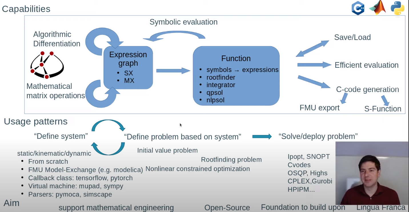
- Functions are defined by a symbolic expression, ODE/DAE integrators, QP solvers, NLP solvers etc
- all function objects in CasADi are multiple matrix-valued input, multiple, matrix-valued output
- converting MX to SX might speed up the calculations significantly, but might also cause extra memory overhead
- plugins: conic, dple, expm, importer, integrator, interpolant, linsol, nlpsol, rootfinder
- sensitivity analysis?
- map vs fold
- numerical evaluation of function objects in CasADi normally takes place in virtual machines
- “black box” function
- lookup-tables:
interpolant - shooting (=explicit integration) vs collocation (=implicit integration )
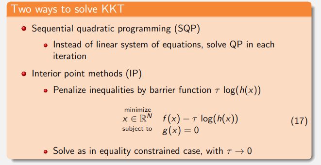
ipopt implements an primal-dual interior-point/barrier line-search filter method.
nlp formulation:
\[\begin{array}{cl} \displaystyle \min_{x \in \mathbb{R}^n} & f(x) \\ \text { s.t. } & g^L \leq g(x) \leq g^U \\ & x^L \leq x \leq x^U \end{array}\]convert to:
\[\begin{array}{cl} \displaystyle \min_{x \in \mathbb{R}^n} & f(x) \\ \text { s.t. } & c(x)=0 \\ & x \geq 0 . \end{array}\]ipopt considers the auxiliary barrier problem:
\[\begin{array}{ll} \displaystyle \min_{x \in \mathbb{R}^n} & \varphi_\mu(x)=f(x)-\mu \sum_{i=1}^n \ln \left(x_i\right) \\ \text { s.t. } & c(x)=0 \end{array}\]first-order optimality conditions:
\[\begin{aligned} \nabla f(x)+\nabla c(x) y-z & =0 \\ c(x) & =0 \\ X Z e-\mu e & =0 \\ x, z & \geq 0 \end{aligned}\]newton step is computed from:
\[\left[\begin{array}{cc} W_k+X_k^{-1} Z_k+\delta_x I & \nabla c\left(x_k\right) \\ \nabla c\left(x_k\right)^T & 0 \end{array}\right]\left(\begin{array}{c} \Delta x_k \\ \Delta y_k \end{array}\right)=-\left(\begin{array}{c} \nabla \varphi_\mu\left(x_k\right)+\nabla c\left(x_k\right) y_k \\ c\left(x_k\right) \end{array}\right)\]where $W_k$ is the Hessian of the Lagrangian function.
computes maximum step sizes as the largest $\alpha$ satisfying
\[x_k+\alpha_k^{x, \max } \Delta x_k \geq(1-\tau) x_k, \quad z_k+\alpha_k^{z, \max } \Delta z_k \geq(1-\tau) z_k\]finally
\[x_{k+1}=x_k+\alpha_{k, l}^x \Delta x_k, \quad y_{k+1}=y_k+\alpha_{k, l}^x \Delta y_k, \quad z_{k+1}=z_k+\alpha_k^{z, \max } \Delta z_k\]once the optimality conditions for the barrier problem are sufficiently satisfied, $\mu$ is decreased.
feasibility restoration phase: which temporarily ignores the objective function, and instead solves a different optimization problem to minimize the constraint violation $\Vert c(x)\Vert_1$.
ipopt iteration output
| col # | header | meaning |
|---|---|---|
| 1 | iter | iteration counter $k$ ( $\mathrm{r}$ : restoration phase) |
| 2 | objective | current value of objective function, $f\left(x_k\right)$ |
| 3 | inf_pr | current primal infeasibility (max-norm), $\Vert c\left(x_k\right)\Vert_{\infty}$ |
| 4 | inf_du | current dual infeasibility (max-norm), $\Vert$ Eqn. $(5 a) \Vert_{\infty}$ |
| 5 | $\lg (\mathrm{mu})$ | $\log _{10}$ of current barrier parameter $\mu$ |
| 6 | $\Vert d\Vert$ | max-norm of the primal search direction, $\left\Vert\Delta x_k\right\Vert_{\infty}$ |
| 7 | $\lg (\mathrm{rg})$ | $\log _{10}$ of Hessian perturbation $\delta_x\left(–:\right.$ none, $\left.\delta_x=0\right)$ |
| 8 | alpha_du | dual step size $\alpha_k^{z, \max }$ |
| 9 | alpha_pr | primal step size $\alpha_k^x$ |
| 10 | ls | number of backtracking steps $l+1$ |
options
- termination
- output
- initialization: interior point method requires that all variables lie strictly within their bounds
- problem modification: ipopt relaxes all bounds (including bounds on inequality constraints) by a very small amount (on the order of $10^{−8}$) before the optimization is started
cite: https://groups.google.com/g/casadi-users/c/4Jq6SN4VKak
An SQP method might need fewer iterations than a nonlinear interior point method (like IPOPT), but each iteration is much more expensive since you’re solving a QP instead of a linear system of equations. That’s why an SQP often makes sense if your function evaluations (including derivative calculations) are very expensive, as is often the case with shooting type methods for optimal control. If function evaluations are cheap (typical for direct collocation type methods), an IP method like IPOPT will probably work better. That being said, an SQP method is also easier to hot-start, which is important for NMPC.
For the kind of problems I try to solve (large and very sparse) I found that the most important settings are (in order): algorithm, linear solver, barrier parameter update strategy For (1) I use interior-point methods; anyway, you only have to consider options of (1) if you have a choice (e.g., in Knitro you can choose between interior-point methods and active-set methods, but I think for Ipopt there’s only one method available AFAIK). For (2), I usually go with HSL MA57. MA27 is a bit slow and outdated. For (3), which is only relevant for barrier methods, I go with “adaptive” updates.
ref